Transformers for Time-series Forecasting
Code: https://github.com/nklingen/Transformer-Time-Series-Forecasting
This article will present a Transformer-decoder architecture for forecasting on a humidity time-series data-set provided by Woodsense . This project is a follow-up on a previous project that involved training an simple LSTM on the same data-set. The LSTM was seen to suffer from “short-term memory” over long sequences. Consequently, a Transformer will be used in this project, which outperforms the previous LSTM implementation on the same data-set.
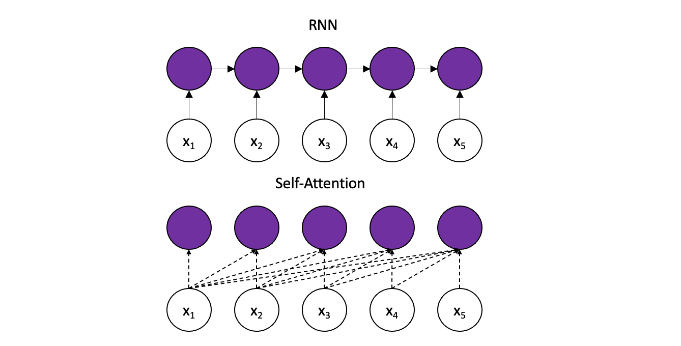
LSTMs process tokens sequentially, as shown above. This architecture maintains a hidden state that is updated with every new input token, representing the entire sequence it has seen. Theoretically, very important information can propagate over infinitely long sequences. However, in practice, this it not the case. Due to the vanishing gradient problem, the LSTM will eventually forget earlier tokens.
In comparison, Transformers retain direct connections to all previous timestamps, allowing information to propagate over much longer sequences. However, this entails a new challenge: the model will be directly connected to an exploding amount of input. In order to filter the important from the unimportant, Transformers use an algorithm called self-attention.
Self-Attention
In psychology, attention is the concentration of awareness on one stimuli while excluding others. Similarly, attention mechanisms are designed to focus on only the most important subsets of arbitrarily long sequences, that are relevant to accomplish a given task.¹
Concretely, the model must decide what details from previous tokes are relevant for encoding the current token. The self-attention block encodes each new incoming input with respect to all other previous inputs, laying focus based on a calculation of relevancy with respect to the current token.
Self-attention is explained in detail in Jay Alammars’ Illustrated GP2 and Illustrated Transformer articles. Additionally, the original paper can be found here. A brief overview is provided below.
- Create Query, Key, and Value Vectors:
Each token generates an associated query, key, and value. The query of the current token is compared to the keys of all other tokens, in order to decide their relevance with respect to the current token. The value vector is the true representation of a given token, that is used in creating the new encoding. During training, the model gradually learns these three weight matrices that each token is multiplied by to generate its corresponding key, query, and value. - Calculate the self-attention score:
The self-attention score is the measure of relevance between the current token and any other token that has previously been seen in the sequence. It is calculated by computing the dot product between the query vector of the current token with the key vector of the token being scored. High scores indicate high relevancy, while low scores indicate the opposite. The scores are then passed through a softmax function, such that they are all positive and add to 1. At this step, the self-attention score can be seen as a percentage of total focus that is given to a token in the sequence, in encoding the current token. - Encoding the current token accordingly:
Words that had a high softmax value in the previous step should contribute more highly to the encoding of the current token, while words with a low score should contribute very little. To accomplish this, each value vector is multiplied by its softmax score. This keeps the original value intact, but scales the overall vector in line with its relative importance for the current token. Finally, all of the scaled values are summed together to produce the encoding of the current token.

As the three steps consist of matrix operations, they can be optimised as follows:

Positional Encoding
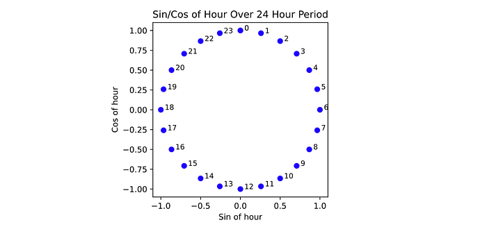
There is also a second challenge that needs to be addressed. The time series is not processed sequentially; thus, the Transformer will not inherently learn temporal dependencies. To combat this, the positional information for each token must be added to the input. In doing so, the self-attention block will have context of relative distance between a given time stamp and the current one, as an important indicator of relevance in self-attention.
For this project, the positional encoding was achieved as follows: the timestamp was represented as three elements — hour, day, and month. To represent each datatype truthfully, each element was decomposed into a sine and cosine component. In this way, December and January are close spatially, just as the months occur close temporally. This same concept is applied to hours and days, such that all elements are represented cyclically.
Implementing the Transformer-decoder
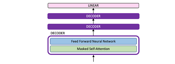
In a vanilla transformer, the decoder consists of the following three blocks: first a masked self-attention block, then an encoder-decoder block, and finally a Feed Forward block. The implementation in this paper draws inspiration from GPT2’s implementation of a decoder-only Transformer, as seen in the figure below. Three of these modified decoder blocks are stacked on top of each other, passing the encoding from the previous block as the input to the subsequent block.
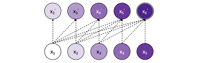
The input to the transformer is a given time series (either univariate or multivariate), shown in green below. The target is then the sequence shifted once to the right, shown in blue below. That is, for each new input, the model outputs one new prediction for the next timestamp.
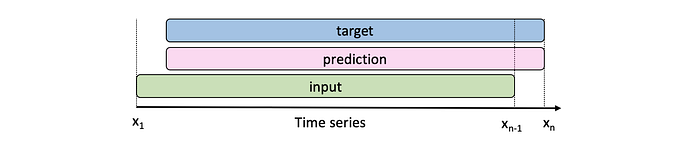
To represent this on a sequence of length 5, for the first input x1, the model will output its prediction for the upcoming token: x2'. Next, it is given the true x1 and x2, and predicts x3', and so forth. At each each new step, it receives all of the true inputs prior in the sequence, to predict the next step. Hereby, the output vector of the model will be the predicted tokens x2', x3', x4', x5', x6'. This is then compared to the true values x2, x3, x4, x5, x6 to train the model, wherein each output token contributes equally to the loss.
Masked Self-Attention
To achieve the model demonstrated above, a mask must be used to ensure that the model only has access to the tokens coming prior in the sequence at each step. Concretely, before the softmax function is applied, all tokens coming after the token currently being attended to are masked, to prevent the model from cheating by looking ahead. When applying the soft-max, these future values will get 0% importance, consequently preventing any information from bleeding through.
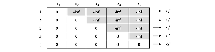
As a final note, the above description has indicated sequential steps in the calculations, for simplicity. In actuality, the calculations are done at the same time in the matrix computations.
Scheduled Sampling
The concept of feeding the model the true value at each new step, rather than the last predicted output, is known as teacher forcing. Just as a student preparing for an exam with his teacher looking over his shoulder, the model learns quickly as its mistakes are instantly corrected. In other words, it never goes “too far off track” before it is corrected.²
The drawback with teacher forcing is that at each new prediction, the model may make minor mistakes, but it will in any case receive the true value in the next step, meaning that these mistakes never contribute significantly to the loss. The model only has to learn how to predict one time step in advance.
However, during inference, the model now must predict longer sequences, and can no longer rely on the frequent corrections. In each step, the last prediction is appended as new input for the next step. Hereby, minor mistakes that were not critical during training quickly become amplified over longer sequences during inference.³ In the previous analogy, this can be likened to the student going to the exam, having never taken a practice test without the aide of his teacher beside him.
A basic problem in teacher forcing emerges: training becomes a much different task than inference. To bridge this gap between training and inference, the model needs to slowly learn to correct its mistakes. The task of transitioning the model between training and inference thus becomes to gradually feed the model more of its predicted outputs, rather than the true values.
Moving too quickly towards inference in the early epochs — sampling too heavily from the model’s predicted output — would result in random tokens, since the model has not yet had the opportunity to train, thereby causing a slow convergence. On the other hand, not moving quickly enough towards inference in the last epochs — sampling too little — will make the gap too large between training and inference, meaning that a model that performs well during training will drastically drop in performance during inference.
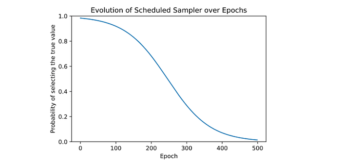
In order to gently bridge this gap, a sampling method is used, inspired by Bengio’s “Scheduled Sampling for Sequence Prediction with Recurrent Neural Networks”. The sampling rate evolves over time, starting with a high probability of selecting the true value initially, as in classical teacher forcing, and gently converging towards sampling purely from the models output, to simulate the inference task. Different schedules are proposed in the paper, of which inverse sigmoid decay was chosen for this project. In these last epochs, when the model samples many of its own predictive values successively, the model ideally learns to prevent its small mistakes from accumulating, as it now is penalized much more highly.
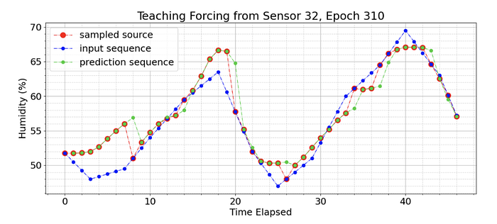
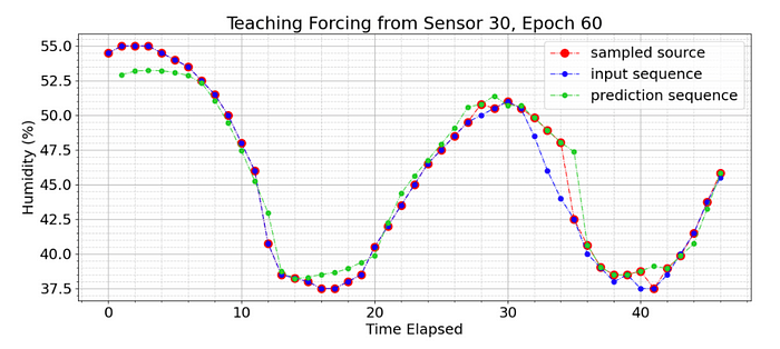
Applying this technique to the model yields results shown below during training at epoch 310 of 500. The blue dots show the true input. The red dots indicate the value chosen as input for the next step — whether the true input or the prediction from the last step. The green dots are the model’s predictions, given only the previous red dots as input. At epoch 310, the model samples only 20% of it’s values from the true input, the other 80% are its own predictions that are built upon, as shown in the inverse sigmoid decay graph above. It is seen that the model is “corrected” each time the sampler selects the true input again.
For example, at timestamp 20, the model had moved significantly off track and predicted a humidity of 65%. The sampler selected the true output as the next input, and the model succeeded in correcting itself almost perfectly in the subsequent timestamp 21.
We see that the model performs poorly in the beginning of the sequence. This is intuitive, considering the model is predicting with very little knowledge of the specific sequence. Training with the scheduled sampler that kicks in early in the sequence was demonstrated to confuse the model, as it is penalized for poor predictions in cases where it does not have sufficient input to understand patterns in the data yet. To correct this, a threshold is set on the scheduled sampler, ensuring that only true values are used for the first 24 time-stamps, representing one full day of data, before the scheduled sampler kicks in at the normal rate demonstrated in the inverse sigmoid graph, correlated with the epoch.
Results
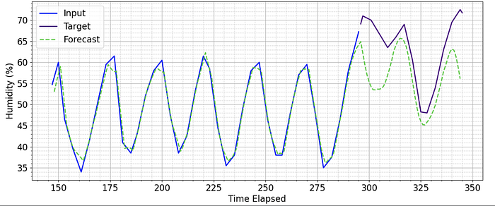
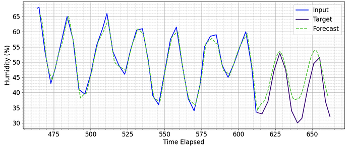
As demonstrated below, this model succeeds in reasonable predictions for a forecast window of 50 timestamps.
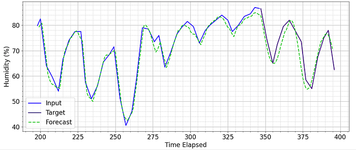

In the cases where it does shift off track over time, it produces convincing predictions that show a deeper understanding of the data.
This article discusses a simple Transformer-decoder architecture for forecasting on an industry dataset. For resources to current SoTA research for Transformers in Time Series, please see Transformers in Time Series: A Survey.
¹ Aston Zhang, Zachary C. Lipton, Mu Li, and Alexander J. Smola, Dive into Deep Learning, 2019 https://d2l.ai/chapter_attention-mechanisms/index.html
² Jason Brownlee,“What is teacher forcing for recurrent neural networks?,” https://machinelearningmastery.com/teacher-forcing-for-recurrent-neural-networks/, Dec 2017
³ Samy Bengio, Oriol Vinyals, Navdeep Jaitly, and Noam Shazeer, “Scheduled sampling for sequence prediction with recurrent neural networks,” CoRR, vol. abs/1506.03099, 2015. https://arxiv.org/pdf/1506.03099.pdf